For anyone who hasn’t seen part 1 of this series, it is available here: Part One – The Event.

Recap

Datalytyx attended the Microsoft AI Hackathon in October 2018. This was an educational exercise and an opportunity for us to learn from the very knowledgeable Microsoft solutions architects who attended the event. We turned up to this event with a dataset containing the Seattle Library collection. Although we didn’t arrive with a plan, after some EDA we found that for each item in the dataset there was a description of the item in string format, however there was no categorization of these items into genres. As there are no categorizations, there are no labels to use in a supervised learning algorithm. Hence we used an unsupervised learning technique, K-means clustering, on the description columns in order to group similar items in the library collection.

Where did we store the data?

Snowflake! – Snowflake is the elastic Enterprise Data Warehouse built for the cloud. As such it provides unlimited concurrency and breathtaking performance while also providing a simple, easy to use web UI. When using Snowflake it is easy to manipulate data using native SQL and quickly share views with other users.

The Data Science Process

Data Science modelling typical consists of 8 layers. The quality of the data at each stage is dependent on the quality of the outputs of each previous stage. If the data preparation at any stage is not adequate then the results of the model will be poor… as they across the pond… “garbage in… garbage out”.

• Understand the data and the problem
• Data Preparation
• Exploratory Data Analysis (EDA)
• Feature Engineering
• Model Benchmarking – mainly for supervised learning as there is labelled data to compare to.
• Model Selection and Tuning
• Operationalise
• Visualisation

What development platform did we use?

Databricks!  – Databricks is a unified analytics platform which handles all analytic processes – from ETL to models, training and deployment. It is powered by Apache Spark^TM. This means that your company can leverage the scalability of Apache Spark^TM, in a collaborative notebook workspace, using the languages your company is familiar with whether it be: python, R, Scala, SQL or Java.

The Model

1. Remove stop words from the text corpus so that the algorithm used will focus on words which convey significantly more meaning. Stop words are natural language words which have very little meaning, such as “and”, “the”, “a”, “an”, and similar words.
2. Stem the text. Stemming is the process of breaking a word down into its root.
3. Tokenise the text. Tokenising is the process of chopping a piece of text into pieces. In this case we want to chop up sentences so that the tokens are individual words.
4. Obtain a Tf-idf matrix for the book description column. Tf-idf is a count of word occurrence per book description with a weighting applied. This weighting is such that words that occur frequently within a book description but not frequently within the corpus receive a higher weighting as these words are assumed to contain more meaning in relation to the description.
5. Compute a measure of the similarity (distance) between each document and other documents in the corpus. This was done as distance = 1 – cosine­_similarity of each book description.
6. Use K-means clustering to group documents by the distance between them. I initialised the model with 5 clusters. Each observation is assigned to a cluster so as to minimize the sum of squares within each cluster. For each cluster, the mean of the clustered observations is calculated and used as the new cluster centroid. Observations are then reassigned to clusters and centroids recalculated in an iterative process until the algorithm reaches convergence.

Results and Visualisation!

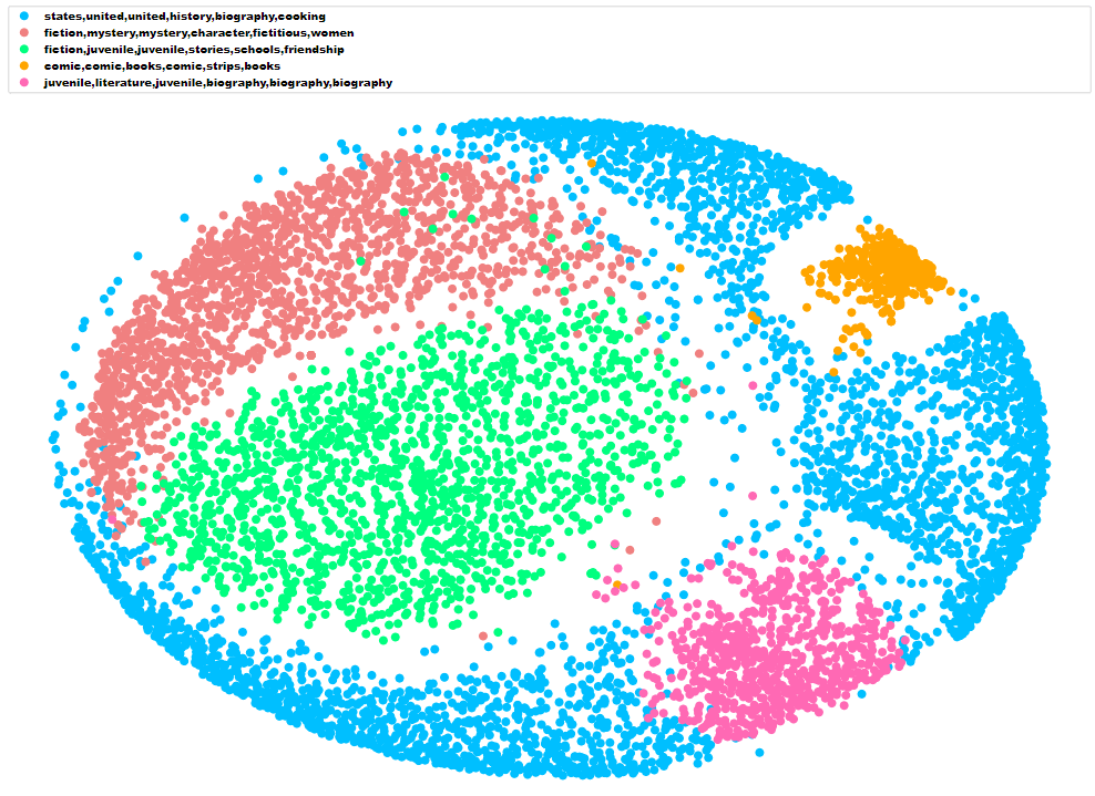
We identified the general theme of each cluster by selecting the six words closest to each cluster centroid.

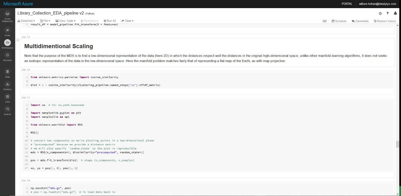
We converted the distance matrix into a 2-dimensional array using multidimensional scaling. This is a technique which allows high dimensional matrices to be visualised in low dimensions such as 2D or 3D. The result of multidimensional scaling is similar to a map-projection from a globe to a 2D map.

Here are the results visualised using the mpld3 python library which allows the creation of D3 plots using matplotlib syntax: