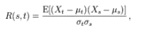
Time series modelling is the process in which data (involving years, weeks, hours, minutes and so on) is analysed using a special set of techniques in order to derive insights. This type of modelling is especially important in the event of having autocorrelated data, where a series is correlated with a delayed copy of itself. One example of this may be the purchasing of a stock. Trading carried out two hours previously may have direct consequences on live trading patterns. The mathematical definition of autocorrelation is defined below:

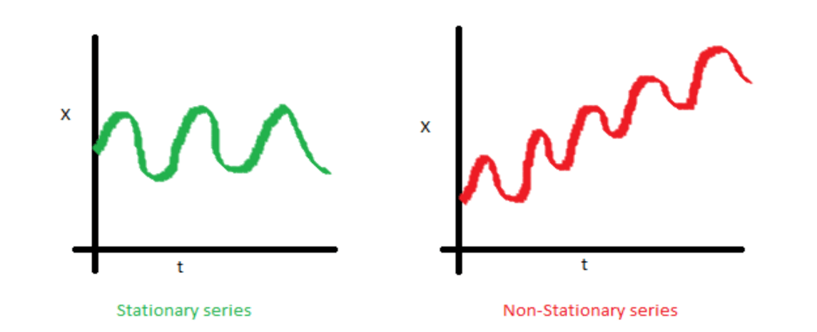
The first step in any time series process is to determine the stationarity of a series, a variable is said to be stationary if its statistical properties such as mean, variance and serial correlation are constant over time. This property makes analysis more straightforward as one can predict statistical properties will remain similar to what they’ve been in the past. An example of a non-stationary series vs stationary series can be seen below:

The reason stationarity has been mentioned is due to its key importance in time series analysis, a series must be classed as stationary before any time series model can be fitted to it. It is often the case with real world data that series are non-stationary and so a set of mathematical techniques have been devised to convert these to stationary. These shall now be discussed in the following section.

Stabilising a non-stationary series

Differencing is the process of computing the differences between consecutive observations, this process can stabilize the mean of a time series by removing changes in the level of a time series. A mathematical representation of differencing is shown below:

For n observations, the differenced series will only have n-1 observations as it is not possible to calculate a difference for the first element of a series. In other words, every time differencing occurs an element is lost. In some cases simply differencing once is not enough to produce the required stationary series, in this case second order differencing is required as shown below:

Here the change in changes would be modelled, as well as there being two less data points belonging to the series. In most cases second order differencing is sufficient to make a series stationary, it is widely recommended to never go beyond seconder differencing.

Unit Root Testing and ARMA Modelling

A statistical method for inferring whether differencing is required on time series is to use a unit root test. There are many different types of unit root tests. The most common and the one that shall be discussed here is the Dickey-Fuller test. This test takes the first difference of a series and then tests the null hypothesis of whether the series has a unit root. If the null hypothesis is accepted then differencing is not required.

Once the stationarity of the series is known or has been taken care of, a method is needed to begin forecasting on the data. ARMA models are one such common way to forecast on stationary time series data. The AR component stands for Auto Regressive while MA stands for moving average. As already explained, auto regressive suggests a series current points to be dependent on previous points. For instance, a nations GDP x(t) is likely to be dependent on last year’s GDP x(t-1). This relationship can be formally written as:

A moving average model is related more to sharp spikes in the time series data and can be modeled by:

In order to determine between an AR and a MA series an auto-correlation function (ACF) plot can be used. This is a plot of total correlation between different lag functions. Also the partial autocorrelation function (PACF) can be used alongside this. The PACF is the correlation between two lags irrespective of other lags in the series. Below are two examples of these two charts.

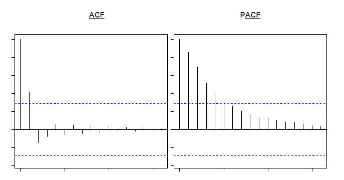
Each bar represents the correlation between the original series and its kth lag. The first bar is always equal to one as this is simply measuring the variable correlated with itself. The blue line apparent in any plot represents statistically significant values other than 0, meaning any bars underneath this threshold are not statistically significant. The method to distinguish between AR and MA processes comes from observing which graph falls below this line first. If the PACF graph becomes insignificant before the ACF plot then the series is mostly an AR process. For instance, in the top two images the PACF becomes insignificant after the second lag, meaning it is an AR(2) process. On the other hand in the bottom images the ACF plot becomes insignificant after the 2^nd bar, meaning it is mostly a MA(2) process.

Forecasting

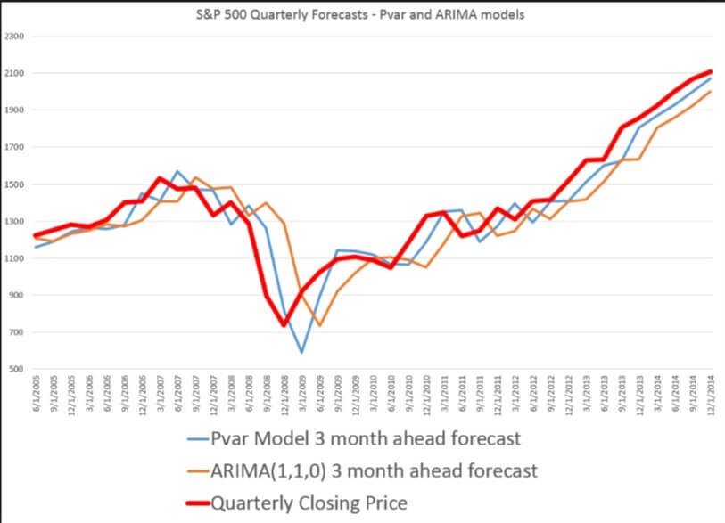
Once is has been determined which type of series is being analysed an ARIMA or ARMA model can be fitted. The ARIMA model comes in ARIMA (p ,d, q), where p and q are the levels of AR and MA respectively. The parameter d stands for how many times of the series has been differenced. For instance a series which is an AR(1) process and has been differenced once would be modelled using an ARIMA(1,1,0) model. The following plot demonstrates a forecasting example.

Accurate forecasting is becoming increasingly important for organisations that use time series data to reduce costs or prepare strategies for increasing revenue. Having an accurate model can be the difference between the success or failure of a business, so it’s vital that the appropriate model is used.